When it comes to CFP® exam prep, investments are one of the many areas that may give you some difficulty, particularly topics such as the Sharpe and Treynor ratios. In fact, investments are one of the toughest areas to teach during a CFP® review course because of the limited amount of time there is for instruction. Luckily, the Board provides investment formulas, but let’s step back and get a grasp of the fundamentals so we can see the big picture and then zoom in on the particulars with a greater understanding and ultimately much higher degree of confidence answering test questions.
Overview
When Harry Markowitz published “Portfolio Selection” in the Journal of Finance back in 1952 and explained his Modern Portfolio Theory (MPT), little did he know how influential his work would become. He also was unaware of how much angst he would cause for thousands of Certified Financial Planner™ exam candidates! In a nutshell, MPT tells us there is an optimal return an investor should expect on a portfolio for a given amount of risk that is being taken. It’s imperative you remember this because it will help you in answering many of the investment questions on the Certified Financial Planner™ exam.
How Do We Measure Risk?
When it comes to measuring risk, we need to understand that it’s made up of two components: systematic risk and unsystematic risk. In a follow-up post, we’ll examine these components more deeply, but for now you need to remember that systematic risk and unsystematic risk combine to make up total risk. But what does total risk actually mean? In the investment world, total risk is the potential for loss AND gain – not simply the potential for loss.
So how do we measure total risk? We measure it by assigning a number to it, and that number is known as the standard deviation. The standard deviation tells us how far an investment’s actual return will vary from its expected return during a particular timeframe (typically one year). So let’s say you’re considering buying XYZ stock and for the past 100 years, XYZ has returned an average of 8%. Therefore, we have enough data to suggest that for a given year, we should expect a return of 8%. But we know that XYZ stock is not going to return exactly 8% every single year and as an investor or portfolio manager, you’d like to know by how much and what percentage of the time XYZ will deviate from 8%; the standard deviation provides that answer.
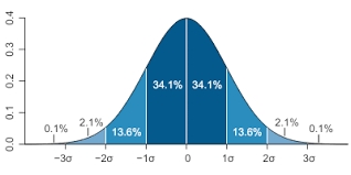
Taking it a step forward, if we examine all of XYZ’s returns for the past 100 years, we notice that 68.2% of the time we get a return of between 6% and 10%, giving us a standard deviation of 2%. We also observe that 95.45% of the time the investment return of XYZ stock is between 4% and 12%, or two standard deviations and 99.73% of the time, we observe a return of between 2% and 14%, or three standard deviations.

We can see from the chart above that the entire area shaded in dark blue is one standard deviation. If the chart represented all of XYZ’s returns observed over our given timeframe of 100 years, we’d notice that 68.2% of the returns fall into the blue-shaded area. The areas shaded in dark blue and lighter blue comprise two standard deviations, while the areas shaded in dark blue, lighter blue and the lightest blue make up three standard deviations.
Although very basic in explanation, if you’re new to the world of investment management, this post should help you as you continue with your CFP® exam prep. As mentioned, I will be addressing a host of investment-related topics and in greater detail in future posts.